Transformer简介

自注意力机制

现在主流的序列模型都是基于复杂的循环神经网络或者是卷积神经网络构造而来的Encoder-Decoder模型,并且就算是目前性能最好的序列模型也都是基于注意力机制下的Encoder-Decoder架构。为什么作者会不停的提及这些传统的Encoder-Decoder模型呢?接着,作者在介绍部分谈到,由于传统的Encoder-Decoder架构在建模过程中,下一个时刻的计算过程会依赖于上一个时刻的输出,而这种固有的属性就限制了传统的Encoder-Decoder模型就不能以并行的方式进行计算。谷歌2017年所发表的一篇论文,名字叫做”Attention is all you need“,在这篇论文中,作者首次提出了一种全新的Transformer架构来解决这一问题。当然,Transformer架构的优点在于它完全摈弃了传统的循环结构,取而代之的是只通过注意力机制来计算模型输入与输出的隐含表示,而这种注意力的名字就是大名鼎鼎的自注意力机制(self-attention)。

image-20211113200639554

总体来说,所谓自注意力机制就是通过某种运算来直接计算得到句子在编码过程中每个位置上的注意力权重;然后再以权重和的形式来计算得到整个句子的隐含向量表示。最终,Transformer架构就是基于这种的自注意力机制而构建的Encoder-Decoder模型。

SelfAttention

在论文中作者说道,注意力机制可以描述为将query和一系列的key-value对映射到某个输出的过程,而这个输出的向量就是根据query和key计算得到的权重作用于value上的权重和。

1
An attention function can be described as mapping a query and a set of key-value pairs to an output, where the query, keys, values, and output are all vectors. The output is computed as a weighted sum of the values, where the weight assigned to each value is computed by a compatibility function of the query with the corresponding key.

\(Attention(Q,K,V)=softmax(\frac{QK^T}{\sqrt{d_k}})V\)

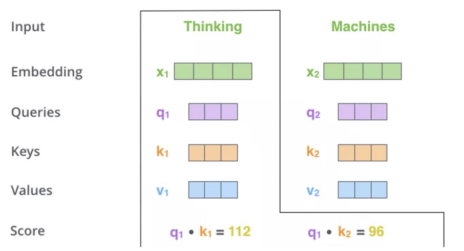
  • 首先,对于输入序列的每个单词,它都有三个向量编码,分别为:Query、Key、Value。这三个向量是用embedding向量与三个矩阵( \(W^Q,W^k,W^V\)​)相乘得到的结果。这三个矩阵的值在BP的过程中会一直进行更新。
  • 第二步计算Self-Attention的分数值,该分数值决定了当我们在某个位置encode一个词时,对输入句子的其他部分的关注程度。这个分数值的计算方法是用该词语的Q与句子中其他词语的Key做点乘。以下图为例,假设我们在为这个例子中的第一个词“Thinking”计算自注意力向量,我们需要拿输入句子中的每个单词对“Thinking”打分。这些分数决定了在编码单词“Thinking”的过程中重视句子其它部分的程度。
image-20211113203629321
  • 再对每个分数除以 \(\sqrt{d}\)​(d是维度),之后做softmax。
image-20211113203726025
  • 把每个Value向量和softmax得到的值进行相乘,然后对相乘的值进行相加,得到的结果即是一个词语的self-attention embedding值。
image-20211113203814342

这样,自注意力的计算就完成了。得到的向量就可以传递给前馈神经网络。

MultiHeadAttention

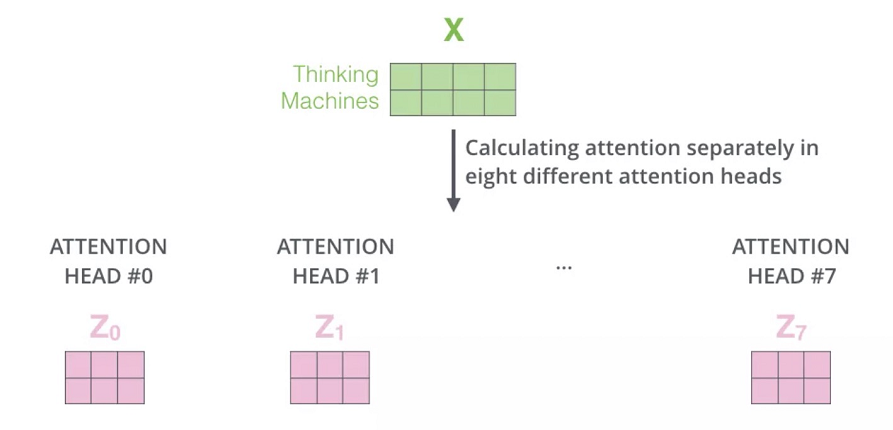
上面我们也提到了自注意力机制的缺陷就是:模型在对当前位置的信息进行编码时,会过度的将注意力集中于自身的位置, 因此作者提出了通过多头注意力机制来解决这一问题。同时,使用多头注意力机制还能够给予注意力层的输出包含有不同子空间中的编码表示信息,从而增强模型的表达能力。

image-20211113203940863

位置编码

Token Embedding

熟悉文本处理的读者可能都知道,在对文本相关的数据进行建模时首先要做的便是对其进行向量化。例如在机器学习中,常见的文本表示方法有one-hot编码、词袋模型以及TF-IDF等。不过在深度学习中,更常见的做法便是将各个词(或者字)通过一个Embedding层映射到低维稠密的向量空间。因此,在Transformer模型中,首先第一步要做的同样是将文本以这样的方式进行向量化表示,并且将其称之为Token Embedding,也就是深度学习中常说的词嵌入(Word Embedding)。

如果是换做之前的网络模型,例如CNN或者RNN,那么对于文本向量化的步骤就到此结束了,因为这些网络结构本身已经具备了捕捉时序特征的能力,不管是CNN中的n-gram形式还是RNN中的时序形式。但是这对仅仅只有自注意力机制的网络结构来说却不行。为什么呢?根据自注意力机制原理的介绍我们知道,自注意力机制在实际运算过程中不过就是几个矩阵来回相乘进行线性变换而已。因此,这就导致即使是打乱各个词的顺序,那么最终计算得到的结果本质上却没有发生任何变换,换句话说仅仅只使用自注意力机制会丢失文本原有的序列信息。

Positional Embedding

论文中提出PE来对序列的位置信息进行编码:

\(PE_{pos,2i}=sin(\frac{pos}{10000^{\frac{2i}{d_{model}}}})\)

\(PE_{pos,2i+1}=cos(\frac{pos}{10000^{\frac{2i}{d_{model}}}})\)

Positional Embedding可以弥补自注意力机制不能捕捉序列时序信息的缺陷。

Transformer网络结构

image-20211113200639554

Encoder

Encoder部分来说其内部主要由两部分网络所构成:多头注意力机制和两层前馈神经网络。同时,对于这两部分网络来说,都加入了残差连接,并且在残差连接后还进行了层归一化操作。对于第2部分的两层全连接网络来说,其具体计算过程为:

\(FFN(x)=max(0,xW_1+b_1)W_2+b_2\)

即对于第1层网络的输出还运用了Relu激活函数。

Decoder

同Encoder部分一样,论文中也采用了6个完全相同的网络层堆叠而成,不过这里我们依旧只是先看1层时的情况。对于Decoder部分来说,其整体上与Encoder类似,只是多了一个用于与Encoder输出进行交互的多头注意力机制。不同于Encoder部分,在Decoder中一共包含有3个部分的网络结构。最上面的和最下面的部分(暂时忽略Mask)与Encoder相同,只是多了中间这个与Encoder输出(Memory)进行交互的部分,作者称之为“Encoder-Decoder attention”。对于这部分的输入,Q来自于下面多头注意力机制的输出,K和V均是Encoder部分的输出(Memory)经过线性变换后得到。而作者之所以这样设计也是在模仿传统Encoder-Decoder网络模型的解码过程。

Transformer的Encoder-Decoder attention中,K和V均是编码部分的输出Memory经过线性变换后的结果(此时的Memory中包含了原始输入序列每个位置的编码信息),而Q是解码部分多头注意力机制输出的隐含向量经过线性变换后的结果。在Decoder对每一个时刻进行解码时,首先需要做的便是通过Q与 K进行交互(query查询),并计算得到注意力权重矩阵;然后再通过注意力权重与V进行计算得到一个权重向量,该权重向量所表示的含义就是在解码时如何将注意力分配到Memory的各个位置上。

示例

MultiHeadAttention

1
2
3
4
5
6
7
8
9
10
11
12
13
14
15
16
17
18
19
20
21
22
23
24
25
class MyMultiheadAttention(nn.Module):
def __init__(self, embed_dim, num_heads, dropout=0., bias=True):
super(MyMultiheadAttention, self).__init__()
"""
:param embed_dim: 词嵌入的维度,也就是前面的d_model参数,论文中的默认值为512
:param num_heads: 多头注意力机制中多头的数量,也就是前面的nhead参数, 论文默认值为 8
:param bias: 最后对多头的注意力(组合)输出进行线性变换时,是否使用偏置
"""
self.embed_dim = embed_dim # 前面的d_model参数
self.head_dim = embed_dim // num_heads # head_dim 指的就是d_k,d_v
self.kdim = self.head_dim
self.vdim = self.head_dim
self.num_heads = num_heads # 多头个数
self.dropout = dropout
assert self.head_dim * num_heads == self.embed_dim, "embed_dim 除以 num_heads必须为整数"
# 上面的限制条件就是论文中的 d_k = d_v = d_model/n_head 条件
self.q_proj_weight = Parameter(torch.Tensor(embed_dim, embed_dim))
# embed_dim = kdim * num_heads
# 这里第二个维度之所以是embed_dim,实际上这里是同时初始化了num_heads个W_q堆叠起来的, 也就是num_heads个头
self.k_proj_weight = Parameter(torch.Tensor(embed_dim, embed_dim))
# W_k, embed_dim = kdim * num_heads
self.v_proj_weight = Parameter(torch.Tensor(embed_dim, embed_dim))
# W_v, embed_dim = vdim * num_heads
self.out_proj = nn.Linear(embed_dim, embed_dim, bias=bias)
# 最后将所有的Z组合起来的时候,也是一次性完成, embed_dim = vdim * num_heads
1
2
3
4
5
6
7
8
9
10
11
12
13
14
15
16
17
18
19
20
21
22
23
24
25
26
27
28
29
30
31
32
33
34
35
36
37
38
39
40
41
42
43
44
45
46
47
48
49
50
51
52
53
54
55
56
57
58
59
60
61
62
63
64
65
66
67
68
69
70
71
72
73
74
75
76
77
78
79
80
81
82
83
84
85
def multi_head_attention_forward(
query, # [tgt_len,batch_size, embed_dim]
key, # [src_len, batch_size, embed_dim]
value, # [src_len, batch_size, embed_dim]
num_heads,
dropout_p,
out_proj_weight, # [embed_dim = vdim * num_heads, embed_dim]
out_proj_bias,
training=True,
key_padding_mask=None, # [batch_size,src_len/tgt_len]
q_proj_weight=None, # [embed_dim,kdim * num_heads]
k_proj_weight=None, # [embed_dim, kdim * num_heads]
v_proj_weight=None, # [embed_dim, vdim * num_heads]
attn_mask=None, # [tgt_len,src_len]
):
# 第一阶段:计算得到Q、K、V
q = F.linear(query, q_proj_weight)
# [tgt_len,batch_size,embed_dim] x [embed_dim,kdim * num_heads]
# = [tgt_len,batch_size,kdim * num_heads]
k = F.linear(key, k_proj_weight)
# [src_len, batch_size,embed_dim] x [embed_dim,kdim * num_heads]
# = [src_len,batch_size,kdim * num_heads]
v = F.linear(value, v_proj_weight)
# [src_len, batch_size,embed_dim] x [embed_dim,vdim * num_heads]
# = [src_len,batch_size,vdim * num_heads]


# 第二阶段:缩放,以及attn_mask维度判断
tgt_len, bsz, embed_dim = query.size() # [tgt_len,batch_size, embed_dim]
src_len = key.size(0)
head_dim = embed_dim // num_heads # num_heads * head_dim = embed_dim
scaling = float(head_dim) ** -0.5
q = q * scaling # [query_len,batch_size,kdim * num_heads]

if attn_mask is not None:
# [tgt_len,src_len] or [num_heads*batch_size,tgt_len, src_len]
if attn_mask.dim() == 2:
attn_mask = attn_mask.unsqueeze(0) # [1, tgt_len,src_len] 扩充维度
if list(attn_mask.size()) != [1, query.size(0), key.size(0)]:
raise RuntimeError('The size of the 2D attn_mask is not correct.')
elif attn_mask.dim() == 3:
if list(attn_mask.size()) != [bsz * num_heads, query.size(0), key.size(0)]:
raise RuntimeError('The size of the 3D attn_mask is not correct.')
# 现在 atten_mask 的维度就变成了3D


# 第三阶段:计算得到注意力权重矩阵
q = q.contiguous().view(tgt_len, bsz * num_heads, head_dim).transpose(0, 1)
# [batch_size * num_heads,tgt_len,kdim]
# 因为前面是num_heads个头一起参与的计算,所以这里要进行一下变形,以便于后面计算。且同时交换了0,1两个维度
k = k.contiguous().view(-1, bsz*num_heads, head_dim).transpose(0,1)
#[batch_size * num_heads,src_len,kdim]
v = v.contiguous().view(-1, bsz*num_heads, head_dim).transpose(0,1)
#[batch_size * num_heads,src_len,vdim]
attn_output_weights = torch.bmm(q, k.transpose(1, 2))
# [batch_size * num_heads,tgt_len,kdim] x [batch_size * num_heads, kdim, src_len]
# = [batch_size * num_heads, tgt_len, src_len] 这就num_heads个QK相乘后的注意力矩阵

# 第四阶段:进行相关掩码操作
if attn_mask is not None:
attn_output_weights += attn_mask # [batch_size * num_heads, tgt_len, src_len]
if key_padding_mask is not None:
attn_output_weights = attn_output_weights.view(bsz, num_heads, tgt_len, src_len)
# 变成 [batch_size, num_heads, tgt_len, src_len]的形状
attn_output_weights = attn_output_weights.masked_fill(
key_padding_mask.unsqueeze(1).unsqueeze(2), float('-inf'))
# 扩展维度,从[batch_size,src_len]变成[batch_size,1,1,src_len]
attn_output_weights = attn_output_weights.view(bsz * num_heads, tgt_len,src_len)
# [batch_size * num_heads, tgt_len, src_len]
attn_output_weights = F.softmax(attn_output_weights, dim=-1)
# [batch_size * num_heads, tgt_len, src_len]
attn_output_weights = F.dropout(attn_output_weights, p=dropout_p, training=training)
attn_output = torch.bmm(attn_output_weights, v)
# Z = [batch_size * num_heads, tgt_len, src_len] x [batch_size * num_heads,src_len,vdim]
# = # [batch_size * num_heads,tgt_len,vdim]
# 这就num_heads个Attention(Q,K,V)结果

attn_output = attn_output.transpose(0, 1).contiguous().view(tgt_len, bsz, embed_dim)
# 先transpose成 [tgt_len, batch_size* num_heads ,kdim]
# 再view成 [tgt_len,batch_size,num_heads*kdim]
attn_output_weights = attn_output_weights.view(bsz, num_heads, tgt_len, src_len)

Z = F.linear(attn_output, out_proj_weight, out_proj_bias)
# 这里就是多个z 线性组合成Z [tgt_len,batch_size,embed_dim]
return Z, attn_output_weights.sum(dim=1) / num_heads # 将num_heads个注意力权重矩阵按对应维度取平均

Transformer的特点

  • 训练时可并行计算
  • Transformer的特征抽取能力也比RNN系列的模型要好,使用了self-attention和多头机制来让源序列和目标序列自身的embedding表示所蕴含的信息更加丰富。